

Table of Content
1. Introduction: Financial Instrument Valuation
The most complex forms of financial valuation are those that depend not on a company’s current assets or income, but on the uncertain future returns of an underlying stock. Share option schemes for employees, convertible debt, warrants, and other hybrid securities are the confluence of financial modelling, probability, and accounting standards – and those who can navigate this space with ease are highly sought after in corporate advisory, corporate finance and audit firms. Financial Instrument Pricing in this area is not just an intellectual exercise: it has real implications for the amount of expense a firm must recognise for its equity-based compensation, whether convertible debt should be classified as debt or equity on the balance sheet, and what dilution effect on existing shareholders will result from changes to the company’s capital structure.
In Australia, the pricing of equity compensation instruments is largely determined by AASB 2 (Share-Based Payment), which requires entities to value equity instruments at their fair value at the grant date and to recognise the resulting expense over the vesting period. The standard requires the use of an option pricing model (usually the Black-Scholes Model or a binomial lattice) and specifies the inputs to be used. However, the implementation of these models in the case of private company instruments, where the prices for the underlying equity are unobservable and where the features of the instruments (such as performance conditions and non-standard vesting periods) add complexity, needs to be done in a way that is more sophisticated than a simple plug-and-play formula in a spreadsheet.
This article aims to be a tool for young and mid-career professionals who work with or around equity compensation, hybrid securities and convertible instruments – whether in audit, corporate advisory, startup financing or M&A – and who wish to gain a better understanding of how these instruments are valued, what the major techniques are, where they are most often misapplied, and what the consequences of misapplication can be. The models discussed here are essential to the practitioner’s financial reporting and transaction services vocabulary.
2. ESOP Valuation: Pricing Employee Equity Compensation
ESOP Valuation, which involves pricing the grant-date fair value of options, performance rights, and other equity issued to employees, is at the forefront of share-based payments accounting under AASB 2. The standard specifies a Grant Date measurement of the Fair Value of Options based on an Option Pricing Models framework that incorporates the exercise price, the current fair value of the underlying shares, the expected volatility of those shares, the risk-free rate, the expected term of the instrument and any expected dividends. For public companies, this data is readily accessible. For private companies – the majority of Australian issuers of ESOP – these inputs need to be determined through a mixture of financial modelling, comparable company research and expert opinion.
The most important input in an ESOP Valuation for a private company is the value of the underlying ordinary shares, since the value of an option is determined by the value of the shares it gives the option holder the right to purchase. This means that, before valuing the option, the current fair value of the underlying ordinary shares must be established – a business valuation exercise in its own right, which demands the same level of rigour and consistency as any other share valuation. For newly established companies with little revenue, this normally involves a weighted average of a range of alternative scenarios (a structured scenario analysis or an option pricing model on the equity value) rather than a traditional EBITDA or DCF Valuation. The Equity Compensation Valuation is therefore embedded in a share valuation exercise, and the underlying quality of the share valuation feeds through to the quality of the option fair value.
The expected volatility input is especially problematic for private companies’ ESOP Valuation. Historical share price volatility is not observable for shares that do not trade on a public exchange, and expected volatility must be inferred from a proxy – usually the historical share price volatility of a peer group of public companies from the same sector. Building a peer group involves both business and statistical considerations: the peers should be comparable in terms of business activity, size and risk profile, and the period over which their volatility is calculated should be representative of the market environment expected over the life of the option. Volatility is a model input that attracts scrutiny from auditors and, as such, practitioners who provide a rationale for their peer selection and the period used to calculate their volatility will have an easier time justifying their inputs than practitioners who simply rely on the sector’s historical volatility.
3. Option Pricing Models: Black-Scholes, Binomial, and Monte Carlo
The Black-Scholes Model is by far the most familiar in Option Pricing Models. For common European-style options (those that can only be exercised at expiry), it remains the most widely used model in both academia and practice. The model provides an analytical formula for the option value that depends on five inputs: the current value of the underlying asset, the exercise price, the risk-free interest rate, the time to expiry and the variance of the underlying asset returns. Its simplicity is appealing – the formula provides a single, deterministic value for the option, given those five inputs – but this simplicity comes with some unrealistic assumptions, especially for employee options where early exercise is prevalent and vesting conditions apply.
When the instrument has American-style exercise features (exercisable at any time before expiry), performance conditions, market-based vesting conditions, or other complications, the binomial lattice model is more flexible. The binomial model builds a lattice of share price paths from the grant date to expiry, assigns probabilities to each node, and then backs out the option’s value at the time of grant. The flexibility of the binomial model is that each node in the tree can include a decision on whether early exercise is the best choice, and performance conditions and vesting schedules can be embedded at the appropriate nodes: the binomial model can handle complexity that the Black-Scholes Model can accommodate only with substantial changes. The cost of this flexibility is a complex computation: a high-resolution binomial tree must be carefully constructed and verified, and the results are more sensitive to the tree’s specification than a closed-form formula.
The Monte Carlo Simulation is the most flexible and computationally complex of the Option Pricing Models. Instead of building a tree of possible outcomes, the Monte Carlo Simulation approach simulates thousands or tens of thousands of possible share price paths over the option’s lifetime, calculates the payoff of the option along each path, and then determines the average of the discounted payoffs as an estimate of the option’s fair value. Monte Carlo Simulation is especially useful for valuing instruments with a share price path-dependent payoff, such as options that are subject to a market-based performance condition (for instance, the options do not vest unless the company’s total shareholder return is greater than that of a benchmark index) or convertible notes with a path-dependent conversion feature. For those practitioners who are developing their technical skills, knowing when the added complexity of Monte Carlo Simulation is justified – rather than being used as a tool to appear clever when a simpler model will do – is a crucial aspect of professional judgment.
4. Convertible Note Valuation and Hybrid Securities
Convertible Note Valuation is a specialised sub-area of Financial Instrument Pricing. The convertible note is both a debt security (it bears interest and has a maturity) and an equity derivative (it gives the holder the right to convert the outstanding principal and interest into equity, either at a specified price or at a price determined based on the next funding round). This means that the Hybrid Securities Valuation exercise must take into account both the value of the debt component and the conversion option, as well as their interaction. The classification and measurement of convertible notes under AASB 9 (Financial Instruments) is based on whether (or to what extent) the conversion feature of the note is considered to have specific characteristics, which affects its categorisation as an instrument held at amortised cost, fair value through profit or loss, or a liability component and an equity component.
The typical method of valuing Convertible Notes in Australian startup and growth companies is to split the instrument into a debt and an option component at the time of issue, and then value each component separately before disclosing the overall fair value as a composite of the two. The debt component is usually valued as a regular bond (discounting the cash flows (interest and principal due) at a discount rate adjusted for the credit risk of the issuing company without conversion rights). The conversion option component is then valued as an option on the underlying equity using an Option Pricing Model framework – the most common approach is the Black-Scholes Model for regular conversion features. Still, Monte Carlo Simulation is used for complex conversion features that include a valuation cap, a discount for future funding rounds, or path-dependent conversion features. The Dilution Impact Analysis is also an important consideration. As a note, conversion dilutes existing shareholders’ shareholdings, reducing the value of the underlying shares at the time of conversion. This dilution effect must be incorporated for convertible instruments issued by companies with complex capital structures.
One common issue in Hybrid Securities Valuation is the valuation of convertible notes issued by early-stage companies, which are structured to defer pricing until a future round. The so-called SAFE (Simple Agreement for Future Equity) and other instruments that offer conversion at a discount to or a cap on the next priced round do not have a conversion price set at issuance, making the Convertible Note Valuation analysis challenging. In such instances, the most suitable method is usually Monte Carlo Simulation, which yields a probability distribution of valuations for the next round, to which the conversion rules are applied. This analysis is as complex as the conversion mechanics are numerous, and Valuation Practitioners faced with these instruments for the first time should discuss them with those more familiar, before settling on a methodology that may not work for the auditor or the investor.
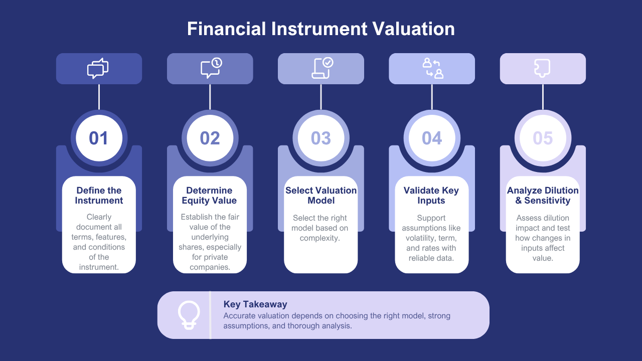
5. Five Key Steps in Financial Instrument Valuation
The five steps described below are common to all types of Financial Instrument Pricing – from relatively simple employee options to the most complex convertible structures – and reflect the way that most experienced practitioners have tackled engagements with the level of rigour required by auditors, boards, and counterparties in transactions.
Step | What It Involves | Common Pitfall |
1. Define the instrument and its features precisely | Document all terms: exercise price, vesting schedule, performance conditions, expiry, early exercise provisions, and any market-based hurdles; for Convertible Note Valuation, document conversion mechanics, interest rate, maturity, and any caps or discounts | Incomplete term documentation leads to model misspecification; practitioners who discover mid-engagement that an instrument has features they have not modelled must redo work that could have been avoided with thorough upfront scoping |
2. Determine the underlying equity value | For private companies, conduct a standalone business valuation to establish the current fair value per share; for ESOP Valuation, this often requires a probability-weighted scenario analysis or an equity allocation model across the capital structure | Using the last round price as the equity value without adjustment is the most common shortcut — and the most commonly challenged by auditors; the last round price reflects the value at a prior date and may not represent current fair value |
3. Select and calibrate the Option Pricing Models framework | Choose between Black-Scholes Model, binomial lattice, and Monte Carlo Simulation based on instrument complexity; for standard vesting options, Black-Scholes is typically sufficient; for path-dependent or market-condition instruments, Monte Carlo Simulation is required | Using the Black-Scholes Model for instruments with complex features, it was not designed to handle produces a Fair Value of Options that is technically wrong; the additional computational effort of the appropriate model is justified by the accuracy of the result |
4. Document and validate all inputs | Source volatility from a well-documented peer group; select a risk-free rate consistent with the instrument’s expected term; apply an expected term (not contractual term) for employee options reflecting historical exercise behaviour and forfeiture estimates; document the basis for every input | The expected term assumption is frequently misstated for employee options; using the full contractual term overstates the Fair Value of Options because employees typically exercise before expiry, and this pattern should be reflected in the model |
5. Perform Dilution Impact Analysis and sensitivity testing | For instruments with potential equity conversion, model the dilution impact on per-share value across conversion scenarios; run sensitivity analysis across key inputs — particularly volatility and expected term — to establish a defensible range and understand what drives the output | Presenting a point estimate without sensitivity analysis leaves the practitioner unable to respond constructively to auditor or counterparty challenges; a well-constructed sensitivity table demonstrates both rigour and awareness of the model’s limitations |
The key judgments in any ESOP Valuation or Convertible Note Valuation of a private company take place during Step 2 – the allocation to equity value. Equity allocation is a particularly knotty issue for companies with preferred shares and liquidation preferences, such as venture-backed companies. In such a case, the ordinary shares held by employees and founders don’t have the same claim on the enterprise value as preferred shares, and the Fair Value of Options must be calculated to reflect the true economics of ordinary shares – not the headline enterprise value divided by the number of outstanding shares. The option-pricing or probability-weighted scenario model used for share allocation is itself a form of Hybrid Securities Valuation, and those who understand the quirks of waterfall distributions and liquidation preferences are well served in this step by the insights this perspective affords, rather than simply performing a per-share arithmetic calculation.
6. Process, Real Cases, and Lessons for Practitioners
The engagement process for Financial Instrument Pricing is not materially different across instrument types, although the steps involved become more complex as the instrument becomes more complex. Knowing how this process works – and where things can go wrong – is as critical as the technical aspects of the models themselves.
Phase 1 | Phase 2 | Phase 3 | Phase 4 |
Instrument Scoping | Equity Value & Input Calibration | Model Build & Valuation | Review, Sensitivity & Reporting |
Collect all instrument term documentation; identify features requiring specialist model treatment; determine underlying equity value approach; confirm applicable accounting standard (AASB 2, AASB 9) | Conduct underlying equity valuation for private company instruments; source and document volatility peer group; determine risk-free rate and expected term; assess Dilution Impact Analysis requirements | Build Black-Scholes Model, binomial lattice, or Monte Carlo Simulation as appropriate; apply ESOP Valuation or Convertible Note Valuation mechanics; compute Fair Value of Options or hybrid instrument value | Run sensitivity tables across volatility, expected term, and equity value; prepare Financial Instrument Pricing report with full input disclosure; support AASB 2 expense calculation and audit review |
An example of the snowball effect of incorrect inputs in ESOP Valuation was a technology company in the growth stage that granted a large block of employee options and valued them using a Black-Scholes model developed by the company. The volatility assumption was based on a single listed peer company – a large-cap technology company whose stable business model and lower growth rate were unlikely to capture the risk profile of the issuing company. After the auditor scrutinised the volatility assumption and requested a peer-group analysis of companies at a similar stage of development, the updated volatility assumption was 35 per cent higher than the original. The change in the Fair Value of Options was significant, necessitating an adjustment to share-based payment expense for the previous period and further audit work. The subsequent remediation cost (in time, money and management resources) far exceeded the cost of using a specialist in the first place.
A more telling example is a startup that issued a Hybrid Securities Valuation challenge in the form of a convertible note with a valuation cap and a 20 per cent discount to the next qualified financing round. The firm’s auditor required a Monte Carlo Simulation to value the conversion option due to the path dependency of the conversion mechanics. The specialist hired to conduct this analysis ran 50,000 scenarios for the next round, applied the cap and discount mechanics to each, and calculated the average discounted payoff of the conversions. The Convertible Note Valuation (broken down between the liability portion and the derivative liability for the conversion option) was significantly different from the estimate provided by management, which had assumed the entire face value of the note was a liability. Proper accounting led to reduced equity and increased liabilities at the time of issue, with fair value changes flowing through the income statement each period. Understanding these issues before issuing convertible instruments can help founders and their finance teams plan for the accounting consequences – rather than finding out too late.
7. Conclusion: Building Technical Depth in Financial Instrument Valuation
Valuation of Financial Instruments for ESOPs, options and convertible notes is very much a crossroads of probability theory, financial modelling and accounting – and those who can address all three competently are among the most technically skilled in the advisory space. The Black-Scholes Model, the binomial lattice, and Monte Carlo Simulation are not alternatives to be selected by choice: each is suitable for a different subset of instrument features, and the decision to select a particular model for a particular instrument is a professional judgement that requires knowledge not simply of the mechanics of each model but the assumptions that each makes and the environments in which each assumption is appropriate.
The focus of developing capability for junior professionals in this area is to build a deeper understanding, starting with the Black-Scholes Model – how it was derived, its inputs, and its shortcomings – and then to the binomial lattice and Monte Carlo Simulation, as instruments with more complex features require more flexible tools. ESOP Valuation under AASB 2 is the most common application encountered in Australia and a great training ground, as the standards requirements are clear, audit scrutiny is predictable, and the variety of instrument types found in practice provides a spectrum of valuation questions that accelerate the development of patterns. The more complex Hybrid Securities Valuation tasks, including Convertible Note Valuation, add a layer of complexity in the interaction of debt and equity and exposure to these instruments – even as a reviewer rather than a primary modeller – speeds up the development of intuition as to when a standard framework will be adequate and when a specialist approach should be sought.
The best advice to advisors who work with companies that issue equity compensation or hybrid instruments is to seek specialist advice before designing and issuing the instruments – not afterwards. The design of an ESOP, the conversion rules of a note, and the performance triggers of a rights plan all impact how the instrument is valued, how the expense or liability is recognised by its issuer, and the Dilution Impact Analysis for existing shareholders. Advisors who have this level of understanding of Equity Compensation Valuation – and who can help their clients understand the accounting and dilution implications of their capital structure decisions before they are finalised – offer a type of value that is both material and uniquely difficult to deliver without specialist technical understanding of Financial Instrument Pricing models and their accounting consequences.

Frequently Asked Questions
Q1. What is business valuation, and why is it important?
Business valuation in Australia is a process of estimating the economic value of a business, ownership interest or a particular asset. It is important because it forms the basis of key business decisions such as purchasing, selling, raising funds and solving conflicts, which gives it a fair and objective basis that everyone can depend on.
Q2. What is a business valuation and an independent expert report?
A business valuation is the analytical process of establishing the value of a business or ownership interest. A separate expert opinion is a step further as it is a formal, objective opinion on whether a particular transaction is fair and reasonable, usually in the interest of shareholders or other interested parties who are considering the proposed transaction.
Q3. What are the circumstances in which an independent expert report is needed?
An independent expert report is usually needed when a fair and objective opinion of a transaction is vital, especially when various parties are involved, and an independent opinion is needed to support transparency, confidence, and informed decision-making in the final outcome.
Q4. What is the average length of a business valuation engagement?
The timeframe depends on business complexity, valuation purpose, and data availability. The less complex interactions can be accomplished in a few weeks, whereas more elaborate or formal assignments can take longer. Anticipated schedules are negotiated and agreed upon at the beginning of any engagement.
Q5. What information is needed to start a valuation engagement?
Typically, we require historical financials, recent management reports, and any available forecasts or business plans. Background information on operations, ownership, and governance is also helpful. To ensure that the process is as simple as possible, a clear information checklist is provided at the start of each engagement.
Q6. How do you give a business valuation of a company that has no history of profitability?
Yes. In the case of new or pre-profit businesses, we use different methods that are not based on past performance but on the prospects. These are scenario-based and market-comparable approaches, which are specific to the nature, stage and circumstances of the business under valuation.
Q6. How do you give a business valuation of a company that has no history of profitability?
Yes. In the case of new or pre-profit businesses, we use different methods that are not based on past performance but on the prospects. These are scenario-based and market-comparable approaches, which are specific to the nature, stage and circumstances of the business under valuation.
Q7. How is business valuation done in Australia?
The most prevalent methodologies are the discounted cash flow analysis, earnings-based multiples, and market benchmarking with similar listed companies or transactions. The decision on which method to use is based on the type of business, the data available, and the intent of the engagement and several methods are usually used and cross-referenced.
Q8. Do your valuations hold up in dispute or litigation?
Yes. Our valuation services in Australia are ready to be presented with the rigour and documentation needed in a formal situation. We provide well-founded conclusions, which are well explained and organised to pass the close scrutiny in disagreements, legal cases or other delicate circumstances.
Q9. What is the value of the business of a privately held company?
For privately owned firms in Australia, valuation is based on financial analysis, earnings normalisation, and market benchmarking due to the absence of a market price. The process takes into consideration the ownership structure, marketability and particular commercial risks to come up with a credible and supportable range of values.
Q10. What are the industries in which you provide your valuation services in Australia?
Our business valuation team has a wide industry focus in Australia and has served the technology, healthcare, professional services, consumer and retail, resources and energy and education industries. Our strategy is shaped by the unique commercial and market features of a particular industry.
Frequently Asked Questions
Q1. What is financial instrument valuation?
Financial instrument valuation determines the fair value of financial assets and liabilities, including shares, derivatives, debt instruments, and convertible securities.
Q2. Why is financial instrument valuation important?
Accurate valuation supports financial reporting, regulatory compliance, investment analysis, risk management, and corporate transactions.
Q3. Which valuation methods are commonly applied?
Depending on the instrument, professionals may use discounted cash flow analysis, option pricing models, market-based approaches, or other recognised valuation techniques.
Q4. Who requires financial instrument valuation?
Businesses, financial institutions, investors, auditors, accountants, and valuation professionals commonly require financial instrument valuations.
Q5. How does professional valuation improve financial reporting?
Professional valuation ensures financial instruments are measured consistently, enhancing transparency, compliance with accounting standards, and stakeholder confidence.